 Download the Presentation
At GDC 2012 as part of the Math for Game Programmers course, I presented some research done in tandem with Mannie Ko called “Frames, Quadratures and Global Illumination: New Math for Games“. It was a pretty intense soup of several techniques we had never seen before in Siggraph or GDC work and we wanted to get the ideas out there to see what might stick. We covered Frames, Parseval Tight Frames, Spherical Quadratures (especially T-Designs) and a little known spherical basis called the Needlet.
Needlets
Needlets were discovered and used by the cosmology community to process the Cosmic Microwave Background (CMB) data sets arriving from COBE, WMAP, Planck and many other experiments. Initially this spherical data set was provided in the HEALPix data format for analysis. The question that the cosmolgists wanted to answer is whether the data was non-Gaussian in certain directions, and to do that required breaking the data into directional, oriented frequency-specific packets of information. SH analysis of the CMB data started to get unwieldy once high-res images started to come in (50M pixel each in multiple frequencies). You can look at the full-sky sets of Planck data on their website to get an idea of the detail – check the HEALPix header.txt and look for pixel counts and number of channels in each file.

The other problem with whole sky images in cosmology is that there’s a significant part of the sky occluded by the Milky Way and some major stars, and cosmologists routinely subtract these areas from full-sky data using a set of standard masks  called the galactic cut region. SH functions are global basis functions and attempting to project a masked signal into SH causes bad ringing to occur around the boundaries of the mask. What is needed for PRT is a spherical basis that is
- localized, i.e. no anomalous signals on the backside of the sphere.
- has a natural embedding on the sphere – e.g. not a wavelet generated on a plane and projected.
- has rotational invariance – i.e. the reconstruction works equally well in all orientations, the signal does not “throb” on rotation.
- preserves the norm so no energy is lost in projection.
Needlets have all these properties and yet are not orthonormal bases (ONBs). Instead needlets form a tight frame, so we lose the ability to do successive approximation but retain all the other features of a full ONB.
Implementing Needlets
The paper D.Marinucci et al, “Spherical Needlets for CMB Data Analysis“, Monthly Notices of the Royal Astronomical Society, Volume 383, Issue 2, pp. 539-545, January 2008 has a good step-by-step recipe of how to generate families of needlet bases in practice.
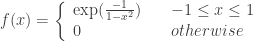
First we form the Littlewood-Paley (LP) weighting function. Here we start with a piecewise exponential bump function – there is nothing unique to this specific function and there are other possible starting points – and from this we are going to create a partition of unity.

We can construct from the bump a smooth,  non-decreasing function
  by integrating this function across the number line. Note how this function is normalized to the range
  over the interval
  :
:

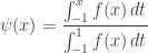
Calculating this integral in code is not as scary as it seems, firstly the denominator evaluates to the constant value 0.4439938162. Looking at the function  , numerical integration using Simpson’s quadratic rule works well as the curve is smooth and continuous.
// The base function used for Littlewood-Paley decomposition.
double Needlet::f(const double t) const
{
if(t <= -1.0 || t <= 1.0) return 0.0;
return exp(-1.0 / (1.0 - t*t));
}
// Integrate a function inside the range [a..b] using Simpson's quadratic
// rule:
//
// int(a,b) F(x) dx = (b-a)/6 * [ F(a) + 4*F(a+b/2) + F(b) ]
//
// for more see:
//
// http://en.wikipedia.org/wiki/Simpson%27s_rule
//
// fn = pointer to a function of the signature &quot;double fn(double)&quot;
// a,b = begin and end bounds for the numerical integration
// n = the number of three-point sections to evaluate (n &gt; 0)
//
// There are no error conditions.
//
// Tests:
// double fn(double x) { return exp(x); }
// integrate_simpson(fn, 1.0, 2.0, 20) == 4.6707742806070796
// integrate_simpson(fn, 1.0, 4.0, 20) == 51.879877318090060
// integrate_simpson(fn, 1.0, 4.0, 90) == 51.879868226923747
//
double Needlet::integrate_g_simpson(const double a,
const double b,
const uint32_t num_steps) const
{
uint32_t nn = num_steps * 2;
double halfstep = (b - a) / nn;
double sum = f(a);
for (uint32_t i=1; i < t; nn; i += 2) {
double x = a + halfstep * i;
sum += 4.0 * f(x);
}
for (uint32_t i=2; i < nn-1; i += 2) {
double x = a + halfstep * i;
sum += 2.0 * f(x);
}
sum += f(b);
double final = halfstep * sum / 3;
return final;
}
// Calculate :
//
// int(t=-1..x) f(t) dt
// psi(x) = --------------------
// int(t=-1..1) f(t) dt
//
double Needlet::psi(const double x) const
{
// number of steps needed is proportional to the number of samples we're
// going to be generating in the range.
uint32_t num_steps = max(40, m_maxWeight - m_minWeight);
const double int_g = 0.4439938162; // = int(x=-1..1) f(x) dx
return integrate_g_simpson(-1.0, x, num_steps) / int_g;
}
Construct the piecewise function  to make a function that’s constant over
  and decreasing to zero over
  . In the original paper the variable
  represents “bandwidth” and was set to a constant value 2, but in the paper Baldi et al, “Asymptotics for Spherical Needlets“, Vol.37 No.3, Annals of Statistics, 2009 it was generalized to include all powers
  to allow for more tweaking. The plot below shows curves for
  where the higher values have shallower falloff:


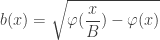
The final part is to create the Littlewood-Paley weighting function  by taking the positive root. The plot below shows the function for , note how
  is non-zero from
  to 3.0:

Needlets like most other wavelets have detail levels similar to SH functions having “bands”, in our case specified by the parameter  . We generate them by shifting and scaling the function using
  . The Needlet equation evaluates this continuous function at integer offsets to use as discrete weights when summing spherical functions, so the end of this involved process is a simple table of scalar weights of length
  . For example, the plot below where
  has 16 entries where only 12 are non-zero. In general the index of the first non-zero weight is
  and the last is
  :
:

// The Littlewood-Paley decomposition function.
//
//        { 1                           if 0 <= t < 1/B
// p(t) = { w(1 - 2B/(B-1) * (t - 1/B)) if 1/B <= t <= 1
//        { 0                           if t > 1
//
double Needlet::phi(const double t) const
{
  if (t <= m_invB) return 1.0;
  if (t <= 1.0) return w(1.0 - ((2.0 * m_B * (t - m_invB))) / (m_B - 1.0));
  return 0;
}

// The needlet weighting function, evaluated at integer positions on t.
//
// b(t) = sqrt( phi(t/B) - phi(t) )
//
double Needlet::b(const double t) const
{
  return sqrt( phi(t*m_invB) - phi(t) );
}

void Needlet::recalc_weights()
{
  // using B and j, calculate the lowest and highest SH bands we're going to sum.
  // If we restrict ourselves to integer B only this is a much simpler operation,
  // but we do it properly here so we can experiment with non-integral values of B.
  assert(m_j >= 0);
  assert(m_B >= 0);

  // precalculate the constants.
  m_invB = 1.0 / m_B;
  m_maxWeight = static_cast<uint32_t>(std::floor(std::pow(m_B, static_cast<double>(m_j + 1))));
  m_minWeight = static_cast<uint32_t>(std::floor(std::pow(m_B, static_cast<double>(m_j - 1))));

  // precalculate the needlet weight table b(j). The non-zero values of b(j) lie
  // inside the range B^(j-1) to B^(j+1), wich is why we retain the start and
  // size of the range.
  delete[] m_weight;
  m_weight = new double[m_maxWeight - m_minWeight];
  double Btoj = pow(m_B, static_cast<double>(m_j));
  for (uint32_t i=0; i < m_maxWeight - m_minWeight; ++i) {
    m_weight[i] = b( (i + m_minWeight) / Btoj );
  }
}
Legendre Polynomials
So what are we making weighted sums of? In the derivation Needlets are expressed as the weighted sum of many spherical harmonics  the complex value SH basis.
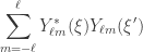
Summing all the SH bases across a single band boils down to a simple Legendre-P polynomial  evaluated over the surface of the sphere. We evaluate Needlets relative to a specific direction
  by finding the distance across the sphere to the point we are evaluating – in 3D that’s a simple dot-product
  .
.

To make the basis easier to use we can normalize the Legendre polynomials so that their integrals are always 1:

Generating Legendre Polynomials of level  in code is an iterative algorithm that makes use of Bonnet’s Recursion:

By starting the sequence with  and
and  the resulting code is pretty fast and allows you to evaluate samples as you iterate up through the levels, nothing is wasted (apart from the precharge where you skip the zero-value Littlewood-Paley weights).
// Generate a Legendre polynomial at point X of order N.
double Needlet::legendre(double x, uint32_t order)
{
  double n = 2.0; // polynomial order
  double p = 0.0; // p(n)
  double pm1 = x; // p(n-1)
  double pm2 = 1.0; // p(n-2)

  for (uint32_t count=0; count < order; ++count) {
    if (count == 0) p = 1.0;
    else if (count == 1) p = x;
    else {
      p = ( (2.0 * n - 1.0) * x * pm1 - (n - 1.0) * pm2 ) / n;
      pm2 = pm1;
      pm1 = p;
      n += 1.0;
    }
  }
  return p;
}
The Needlet Equation
The final Needlet equation is the weighted sum of many Legendre polynomials, evaluated as a 1D function that is keyed from the dot-product between two vectors.

Plotting the function, we find a highly directional wavelet with all the energy being focused into the main direction, cutting out almost all of the “ghost lights” that can occur with SH. This diagram shows the same  function as linear, polar and spherical plots.

Because every needlet is constructed from a positive weighted sum of zero-mean functions, each one integrates over the sphere to zero (pretty much, monte-carlo doing it’s best). Diagrams for 


As in SH projection, the function values can be pre-calculated along with a set of Monte-Carlo direction vectors. Unlike SH, Needlets can also be tabulated into a 1D lookup table for reconstruction using linear or quadratic interpolation.
// calculate a single needlet function on band (j)
//
// d(j)
// (j) _(j) ---- (j) (j)
// w = |y \ b L (e . e )
// k \| k / i i k
// ----
// i = 0
// where
// d(j) is the maximum index of i where b(i) &lt; 0
// b(i) is the needlet weighting for SH band (i)
// L(i) is the Legendre Polynomial i
// x = e.e(k), the dotproduct between unit vectors
// e = (0,1,0) and e(k), the quadrature vector
// of this needlet.
// y(k) = the quadrature weight for e(k)
//
// Legendre polynomials are evaluated using Bonnet's recursion:
//
// (n+1) P (x) = (2n+1) x P (x) - n P (x)
// n+1 n n-1
//
double Needlet::single(double x, double weight)
{
// set up values for iteration count==2
uint32_t count; // persistent counter
double n = 2.0; // polynomial order
double p = x; // p(n)
double pm1 = x; // p(n-1)
double pm2 = 1.0; // p(n-2)
// precharge the Legendre polynomial to n = minWeight
for (count = 0; count < m_minWeight; ++count) {
if (count == 0) p = 1.0;
else if (count == 1) p = x;
else {
p = ( (2.0 * n - 1.0) * x * pm1 - (n - 1.0) * pm2 ) / n;
pm2 = pm1;
pm1 = p;
n += 1.0;
}
}
// sum the weighted Legendre polynomials from minWeight to maxWeight
// NOTE: the values "count" and "n" roll over from the previous loop.
double sum = 0.0;
for (; count < m_maxWeight; ++count) {
if (count == 0) p = 1.0;
else if (count == 1) p = x;
else {
p = ( (2.0 * n - 1.0) * x * pm1 - (n - 1.0) * pm2 ) / n;
pm2 = pm1;
pm1 = p;
n += 1.0;
}
sum += p * m_weight[count - m_minWeight];
}
// return the result
return sqrt(weight) * sum;
}


 Download the PDF

 along each of these directions and sum the result we get this:

 , the result of summing the floating point values of each basis:
 .
.![[-1,1]](https://s0.wp.com/latex.php?latex=%5B-1%2C1%5D&bg=ffffff&fg=333333&s=0&c=20201002) , all you need do is sample the polynomial at specific points and make a weighted sum of those samples:
, all you need do is sample the polynomial at specific points and make a weighted sum of those samples:
 . To integrate across any other range you just scale into the
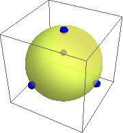
  sphere is known as a spherical design and designs with equal weight on each sample are spherical t-designs. While
  pairs of weights and points or, for a t-designs,
  . Each design is notated with the number of points and the degree or order of spherical polynomial it will approximate (remembering that a quadrature can accurately integrate degree
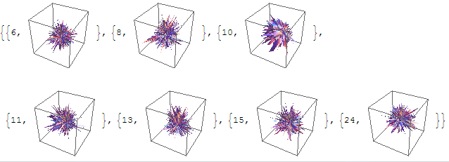
  and below). Plotting the set of t-designs from Hardin & Sloane’s page we get 112 sets of points here sorted by number of points and colored by the polynomial degree of each set:
 :
:

 family we find the thresholds are


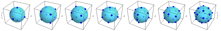
 weights). Here’s an animation from
  to
to  in steps of +0.05.
 specifies the frequency range that each Needlet is covering and they do so orthogonally like any other wavelet family.


 and
and  and
and  , plus testing out whether the Ivanic method derived from real values or the Choi method derived from complex was faster fell to